Please note that the formulas are meant to be applied to a single time series.
The python-cmethods package can apply these formulas to single and
multidimensional data.
The Linear Scaling bias correction technique can be applied on stochastic and
non-stochastic climate variables to minimize deviations in the mean values
between predicted and observed time-series of past and future time periods.
This method requires that the time series can be grouped by time.month.
Since the multiplicative scaling can result in very high scaling factors, a
maximum scaling factor of 10 is set. This can be changed by passing the desired
value to the hidden max_scaling_factor argument.
The Linear Scaling bias correction technique implemented here is based on the
method described in the equations of Teutschbein, Claudia and Seibert, Jan
(2012) “Bias correction of regional climate model simulations for hydrological
climate-change impact studies: Review and evaluation of different methods”
(https://doi.org/10.1016/j.jhydrol.2012.05.052). In the following the equations
for both additive and multiplicative Linear Scaling are shown:
Additive:
In Linear Scaling, the long-term monthly mean (\(\mu_m\)) of the modeled
data \(X_{sim,h}\) is subtracted from the long-term monthly mean of the
reference data \(X_{obs,h}\) at time step \(i\). This difference in
month-dependent long-term mean is than added to the value of time step
\(i\), in the time-series that is to be adjusted (\(X_{sim,p}\)).
The Variance Scaling bias correction technique can be applied only on
non-stochastic climate variables to minimize deviations in the mean and variance
between predicted and observed time-series of past and future time periods.
This method requires that the time series can be grouped by time.month.
Since the the scaling by ratio can result in very high scaling factors, a
maximum scaling factor of 10 is set. This can be changed by passing the desired
value to the hidden max_scaling_factor argument.
The Variance Scaling bias correction technique implemented here is based on the
method described in the equations of Teutschbein, Claudia and Seibert, Jan
(2012) “Bias correction of regional climate model simulations for hydrological
climate-change impact studies: Review and evaluation of different methods”
(https://doi.org/10.1016/j.jhydrol.2012.05.052). In the following the equations
of the Variance Scaling approach are shown:
(1) First, the modeled data of the control and scenario period must be
bias-corrected using the additive linear scaling technique. This adjusts the
deviation in the mean.
The Delta Method bias correction technique can be applied on stochastic and
non-stochastic climate variables to minimize deviations in the mean values
between predicted and observed time-series of past and future time periods.
This method requires that the time series can be grouped by time.month.
Since the multiplicative scaling can result in very high scaling factors, a
maximum scaling factor of 10 is set. This can be changed by passing the desired
value to the hidden max_scaling_factor argument.
The Delta Method bias correction technique implemented here is based on the
method described in the equations of Beyer, R. and Krapp, M. and Manica, A. (2020)
“An empirical evaluation of bias correction methods for paleoclimate simulations”
(https://doi.org/10.5194/cp-16-1493-2020). In the following the equations
for both additive and multiplicative Delta Method are shown:
Additive:
The Delta Method looks like the Linear Scaling method but the important
difference is, that the Delta method uses the change between the modeled
data instead of the difference between the modeled and reference data of the
control period. This means that the long-term monthly mean (\(\mu_m\))
of the modeled data of the control period \(T_{sim,h}\) is subtracted
from the long-term monthly mean of the modeled data from the scenario period
\(T_{sim,p}\) at time step \(i\). This change in month-dependent
long-term mean is than added to the long-term monthly mean for time step
\(i\), in the time-series that represents the reference data of the
control period (\(T_{obs,h}\)).
The multiplicative variant behaves like the additive, but with the
difference that the change is computed using the relative change instead of
the absolute change.
The Quantile Mapping bias correction technique can be used to minimize
distributional biases between modeled and observed time-series climate data. Its
interval-independent behavior ensures that the whole time series is taken into
account to redistribute its values, based on the distributions of the modeled
and observed/reference data of the control period.
The Quantile Mapping technique implemented here is based on the equations of
Alex J. Cannon and Stephen R. Sobie and Trevor Q. Murdock (2015) “Bias
Correction of GCM Precipitation by Quantile Mapping: How Well Do Methods
Preserve Changes in Quantiles and Extremes?”
(https://doi.org/10.1175/JCLI-D-14-00754.1).
The regular Quantile Mapping is bounded to the value range of the modeled data
of the control period. To avoid this, the Detrended Quantile Mapping can be
used.
In the following the equations of Alex J. Cannon (2015) are shown and explained:
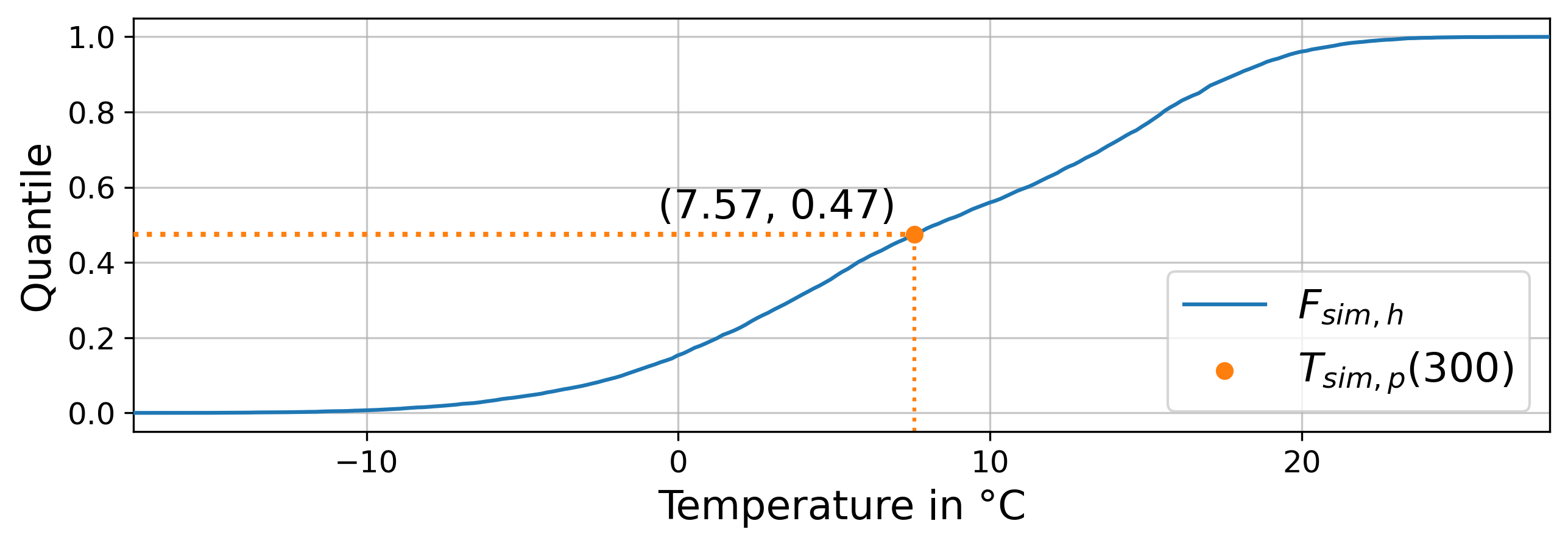
The additive quantile mapping procedure consists of inserting the value to
be adjusted (\(X_{sim,p}(i)\)) into the cumulative distribution function
of the modeled data of the control period (\(F_{sim,h}\)). This
determines, in which quantile the value to be adjusted can be found in the
modeled data of the control period The following images show this by using
\(T\) for temperatures.
Fig 1: Inserting \(X_{sim,p}(i)\) into \(F_{sim,h}\) to determine the quantile value
This value, which of course lies between 0 and 1, is subsequently inserted
into the inverse cumulative distribution function of the reference data of
the control period to determine the bias-corrected value at time step
\(i\).
Fig 1: Inserting the quantile value into \(F^{-1}_{obs,h}\) to determine the bias-corrected value for time step \(i\)
Multiplicative:
The formula is the same as for the additive variant, but the values are
bound to the lower level of zero. The upper and lower boundary can be
adjusted by passing the hidden arguments val_min and val_max.
The Detrended Quantile Mapping bias correction technique can be used to minimize
distributional biases between modeled and observed time-series climate data like
the regular Quantile Mapping. Detrending means, that the values of
\(X_{sim,p}\) are shifted by the mean of \(X_{sim,h}\) before the
regular Quantile Mapping is applied. After the Quantile Mapping was applied, the
mean is shifted back. Since it does not make sense to take the whole mean to
rescale the data, the month-dependent long-term mean is used.
This method must be applied on a 1-dimensional data set i.e., there is only one
time-series passed for each of obs, simh, and simp. This method
requires that the time series can be grouped by time.month.
Since the ratio when applying the multiplicative variant can result in extreme
factors, a maximum scaling factor of 10 is set. This can be changed by passing
the desired value to the hidden max_scaling_factor argument.
The Detrended Quantile Mapping technique implemented here is based on the
equations of Alex J. Cannon and Stephen R. Sobie and Trevor Q. Murdock (2015)
“Bias Correction of GCM Precipitation by Quantile Mapping: How Well Do Methods
Preserve Changes in Quantiles and Extremes?”
(https://doi.org/10.1175/JCLI-D-14-00754.1).
The following equations qre based on Alex J. Cannon (2015) but extended the
shift of \(X_{sim,p}(i)\):
The Quantile Delta Mapping bias correction technique can be used to minimize
distributional biases between modeled and observed time-series climate data. Its
interval-independent behavior ensures that the whole time series is taken into
account to redistribute its values, based on the distributions of the modeled
and observed/reference data of the control period. In contrast to the regular
Quantile Mapping (cmethods.CMethods.quantile_mapping()) the Quantile Delta
Mapping also takes the change between the modeled data of the control and
scenario period into account.
Since the ratio when applying the multiplicative variant can result in extreme
factors, a maximum scaling factor of 10 is set. This can be changed by passing
the desired value to the hidden max_scaling_factor argument.
The Quantile Delta Mapping technique implemented here is based on the equations
of Tong, Y., Gao, X., Han, Z. et al. (2021) “Bias correction of temperature and
precipitation over China for RCM simulations using the QM and QDM methods”.
Clim Dyn 57, 1425-1443 (https://doi.org/10.1007/s00382-020-05447-4). In the
following the additive and multiplicative variant are shown.
Additive:
(1.1) In the first step the quantile value of the time step \(i\) to adjust is stored in
\(\varepsilon(i)\).
(1.2) The bias corrected value at time step \(i\) is now determined
by inserting the quantile value into the inverse cumulative distribution
function of the reference data of the control period. This results in a bias
corrected value for time step \(i\) but still without taking the change
in modeled data into account.
The first two steps of the multiplicative Quantile Delta Mapping bias
correction technique are the same as for the additive variant.
(2.3) The \(\Delta(i)\) in the multiplicative Quantile Delta Mapping
is calculated like the additive variant, but using the relative than the
absolute change.